SIMAPSE is a free, open source and multiplatform species habitat modelling tool written in Python. It uses a feedforward neural network with backpropagation algorithm to build a habitat model with species' data (presence with real or pseudo absences).

SIMAPSE is spatial explicit and accepts ASCII file formats as input data. It has an option to control the production of several models with different sub-sampling methods and it provides full control of the neural network structure and learning parameters.

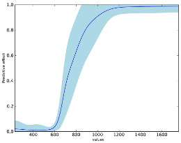
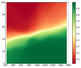
All results are given in text format, easily accessible with multiple softwares. It also provides average predictions in ASCII raster format with associated uncertainties and measures of model fitness. Variable importance and behaviour are assessed with different approaches (profiles, partial derivatives and variable surfaces) and the resulting plots plus text files with raw values are provided.

Download

You can download SIMAPSE here! Unpack the file to any directory. Please read the next section for further instructions on how to run this tool.

NEW VERSION:
The version 1.01 beta is available here. Major changes include a command line interpreter (run "simapse --help" in the terminal to see further details) and the number limit of pseudo-absences was removed. It requires python 2.7 (or previous versions with the argparse module installed).

Instructions

Installation

SIMAPSE is ready to use after unpacking if you have Python in your system. SIMAPSE can build models and text results using only Python core installation. Nevertheless, it depends on few extra python modules to create all graphical results: prediction and uncertainty maps, model fitness and variable importance and behaviour. The general procedure to use the full capabilities of SIMAPSE is similar across different platforms:

• Download python for your system, if you don't have it already installed. SIMAPSE was created with Python version 2.6 and compatible with version 2.7. Soon we will add a version compatible with Python 3.
  
  
• Download and install the following extra modules if you want to generate plots:
  
• NumPy
  
• SciPy
  
• Matplotlib
  
• Python Imaging Library (PIL)
  

Do not forget to download the modules compatible with your Python version and your OS. For instance, if you use a 32bit Windows with Python 2.7, download the file that has win32 and python2.7 in the filename.
If you have trouble finding updated binaries for Windows, here you can find nonofficial binaries - thanks to C. Gohlke! Look for a compatible version with your system (the filename contains amd64 for 64bit systems or win32 for 32bit) and your Python version.


• Run SIMAPSE

If you are using a Linux distribution you may find easier to use the distribution's package management system to install the modules.


How does it work?

The core of SIMAPSE is based on feedforward neural networks with backpropagation learning. Neural networks are artificial neurons connected by adjustable weights, imitating the biological neural networks. This adjustable nature allows processing information and finding complex relationships between inputs and outputs.

The function of the neural networks in SIMAPSE is to learn how the species data is related to the descriptors (raster variables). This is done in the training stage (or learning stage) by presenting the species data and the related descriptors values to the network, so it can adjust the weights connecting neurons by minimizing the difference between the predictive value and the real value (presence, absence or abundance), i.e. minimizing the error. This process of supervised learning is repeated several times (iterations) so the network can find a minimum error in the error surface. While training, each iteration is also compared to a test data (a subset of the original data) to check the overfitting/generalization ability of the network

After the training stage, the iteration of the network with the lowest error is chosen. This trained network will predict species presence (or abundance) in the study area, resulting in a map of probability of occurence. The sub-sampling method will ensure the repetition of these processes several times, to produce a final consensus (average) map between models and an uncertainty associated with the modelling process.


Usage

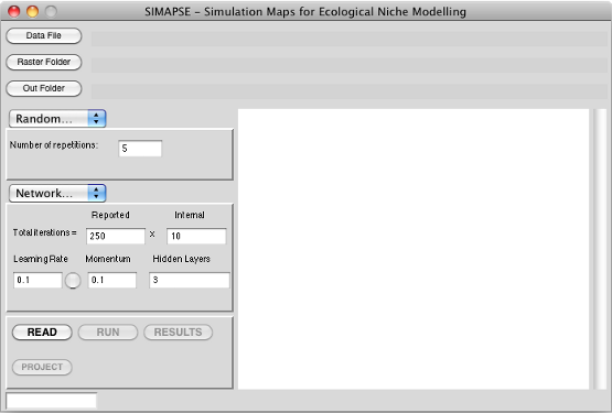
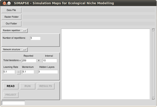
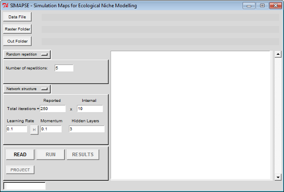
The usage of SIMPASE is straightforward. The graphical user interface is divided in 4 main areas.

• In the top it can be defined the input and output files and directories.
  
• The control options (in the left) are subdivided in the sub-sampling method, modelling options and buttons.
  
• The information text box (in the right) provides all information about the model process (TIP: the text box is editable, you can use it as a notepad to add some notes about the model) and is saved in the output folder as a log text file.
• In the bottom of the graphical interface there is the information panel about the running process.

The common work flow begins by choosing the input data (species data and raster maps as variables) and output directory. The species data should be provided in a text file with semicolon as separator and a header in the first line. The order must be species data, longitude and latitude (column names are arbitrary but the order must be followed). Species data must be 1 for presence, 0 for absence, or with decimals between 0 and 1 for abundance data. Example with presence-only data:

Pres;X;Y
1;1.23;42.12
1;1.92;42.75
1;1.75;42.28
...

The variables must be in the ASCII raster file format. For a correct use, all raster variables must be spatially aligned with the same resolution and clipped by the same mask. Any GIS package with raster support should provide tools to accomplish this. Some of the most used climate data sources are WorldClim and CliMond and CGIAR-CSI.

The next step is to choose the sub-sampling method and the network options. The available sub-sampling methods are:

• random - each set of train and test is chosen randomly
  
• k-fold cross-validation - species data is divided into k-folds and the network is trained k times with k-1 folds against the remaining fold.
• bootstraps - species data is sampled with repetition n number of times (bootstraps) to user-defined dataset size.

The network may be optimized with several options. It is possible to define the number of iterations by choosing the number of internal and reported iterations. The first are hidden iterations by the network and the latter are the number of error reports (shown in the text box) after each cycle of internal iterations. The learning parameters are the learning rate (the allowed amount of learning in each learning cycle) and the momentum (how much the learning amount of the previous cycle can influence the current cycle). The HINT button provides an estimate of error decrease for several learning rates based on the user defined momentum, internal iterations and structure.

The architecture of the network is defined in the structure with number of neurons per layer separated by commas (excluding input and output layers). For example: a structure with 3 hidden layers with 4 neurons in each layer plus input and output is defined by "4,4,4". Keep in mind that simple single layers structures can resolve complex relationships between species presence/absence and variables.

In the Options the user may define the amount of data reserved to test (defined by a percentage of the total data) and, in the case of presence-only data the amount of pseudo-absences to be created - a ratio of pseudo-absences vs. presences - with the default set to 1 (same number of pseudo-absences as presences). The pseudo-absences are randomly chosen in all cells of the given area (defined in each raster variable - see above) for which a presence is not reported. The user may also change the burn-in iterations that are the first learning cycles of the network's training phase. The purpose of this option is to remove the networks that may achieve low errors by random, before any substantial learning.

The users may also filter network results with AUC. With this option activated, for each reported network, it is displayed the train and test AUC with the network train and test errors. By choosing an AUC threshold, only networks that achieve higher AUC will pass to the sorting where the final network is chosen. Very high values increase the chance of refusing all networks, therefore, failing to produce a model, especially with data with very complex relationships.

After defining all parameters, it is possible to start the process with the buttons. The READ button will initiate the reading of species and raster variables and display information about those data. The RUN button starts the modelling process with all the repetitions. TIP: if you are testing the best network to your data, define a low number of iterations and repetitions because the modelling process cannot be cancelled. The RESULTS button will make the final results by calculating the average and standard results of all repetitions and, if you have the extra modules (see installation instructions), will plot all data.

Screenshots

SIMAPSE was tested in Mac OSX, Linux (Ubuntu) and Windows 7/XP (32 and 64 bit versions). This is how it looks in different systems:


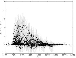
and some of the results:

Credits

SIMAPSE was released under GNU GENERAL PUBLIC LICENSE. See www.gnu.org/licenses or enclosed files in the compressed archive for more details.

Contact:
ptarroso at cibio.up.pt

SIMAPSE was published in Methods in Ecology and Evolution journal. Please cite:

Tarroso, P., Carvalho, S. B. and Brito, J. C. 2012. Simapse - simulation maps for ecological niche modelling. Methods in Ecology and Evolution 3: 787-791.

(last updated: 07-Jul-2014)